Basic example: Simple Linear System

This example demonstrates the basic workflow of using the KKF library with a simple linear dynamical system.

======================================================================
KKF Basic Example: Simple Linear System
======================================================================

System created:
  State dimension: 2
  Measurement dimension: 1
  Discrete time: True

Generating synthetic data...
  Generated 50 timesteps of observations

Setting up Koopman Kalman Filter...
  Number of kernel features: 20
  Prior initial state mean: [0.9 0.4]

Applying Koopman Kalman Filter...
✓ Filter completed successfully!

Solution properties:
  State dimension: 2
  Feature dimension: 20

Estimation errors:
  Mean absolute error: 0.146182
  Max absolute error: 0.252747

Generating plots...
/home/docs/checkouts/readthedocs.org/user_builds/kkf/checkouts/latest/examples/01_basic_linear_system.py:170: UserWarning: Tight layout not applied. The bottom and top margins cannot be made large enough to accommodate all Axes decorations.
  plt.tight_layout()
  Figure saved as 'kkf_basic_example.png'

======================================================================
Example completed successfully!
======================================================================

import numpy as np
import matplotlib.pyplot as plt
from scipy import stats
from sklearn.gaussian_process.kernels import RBF

from kkf import DynamicalSystem, KoopmanOperator, apply_koopman_kalman_filter


def main():
    """Run basic KKF example."""
    print("=" * 70)
    print("KKF Basic Example: Simple Linear System")
    print("=" * 70)

    # System parameters
    nx, ny = 2, 1  # State dimension: 2, Measurement dimension: 1
    dt = 0.1

    # Define linear system dynamics: x[k+1] = A @ x[k]
    A = np.array([[0.9, 0.05], [0.0, 0.95]])

    def f(x):
        """State transition function."""
        return A @ x

    def g(x):
        """Measurement function (observe first state)."""
        return np.array([x[0]])

    # Define noise distributions
    X_dist = stats.multivariate_normal(mean=np.zeros(nx), cov=np.eye(nx))
    dyn_noise_dist = stats.multivariate_normal(
        mean=np.zeros(nx), cov=1e-3 * np.eye(nx)
    )
    obs_noise_dist = stats.multivariate_normal(mean=np.zeros(ny), cov=1e-2 * np.eye(ny))

    # Create dynamical system
    system = DynamicalSystem(
        nx=nx,
        ny=ny,
        f=f,
        g=g,
        dist_X=X_dist,
        dist_dyn=dyn_noise_dist,
        dist_obs=obs_noise_dist,
        discrete_time=True,
    )

    print(f"\nSystem created:")
    print(f"  State dimension: {system.nx}")
    print(f"  Measurement dimension: {system.ny}")
    print(f"  Discrete time: {system.discrete_time}")

    # Generate synthetic measurement data
    print(f"\nGenerating synthetic data...")
    n_timesteps = 50
    x_true = np.zeros((n_timesteps, nx))
    y_meas = np.zeros((n_timesteps, ny))

    # Initial state
    x_true[0] = np.array([1.0, 0.5])
    y_meas[0] = g(x_true[0]) + obs_noise_dist.rvs()

    for t in range(1, n_timesteps):
        x_true[t] = f(x_true[t - 1]) + dyn_noise_dist.rvs()
        y_meas[t] = g(x_true[t]) + obs_noise_dist.rvs()

    print(f"  Generated {n_timesteps} timesteps of observations")

    # Setup Koopman operator
    print(f"\nSetting up Koopman Kalman Filter...")
    n_features = 20
    kernel = RBF(length_scale=1.0)
    koopman_op = KoopmanOperator(kernel, system)

    # Define prior for initial state
    x0_prior = np.array([0.9, 0.4])
    initial_prior = stats.multivariate_normal(
        mean=x0_prior, cov=0.1 * np.eye(nx)
    )

    print(f"  Number of kernel features: {n_features}")
    print(f"  Prior initial state mean: {x0_prior}")

    # Apply Koopman Kalman Filter
    print(f"\nApplying Koopman Kalman Filter...")
    solution = apply_koopman_kalman_filter(
        koopman_operator=koopman_op,
        observations=y_meas,
        initial_distribution=initial_prior,
        n_features=n_features,
        optimize=False,
        noise_samples=50,
    )

    print(f"✓ Filter completed successfully!")
    print(f"\nSolution properties:")
    print(f"  State dimension: {solution.get_state_dimension()}")
    print(f"  Feature dimension: {solution.get_feature_dimension()}")

    # Compute errors
    state_error = np.linalg.norm(solution.x_plus - x_true, axis=1)
    mean_error = np.mean(state_error)
    max_error = np.max(state_error)

    print(f"\nEstimation errors:")
    print(f"  Mean absolute error: {mean_error:.6f}")
    print(f"  Max absolute error: {max_error:.6f}")

    # Visualization
    print(f"\nGenerating plots...")
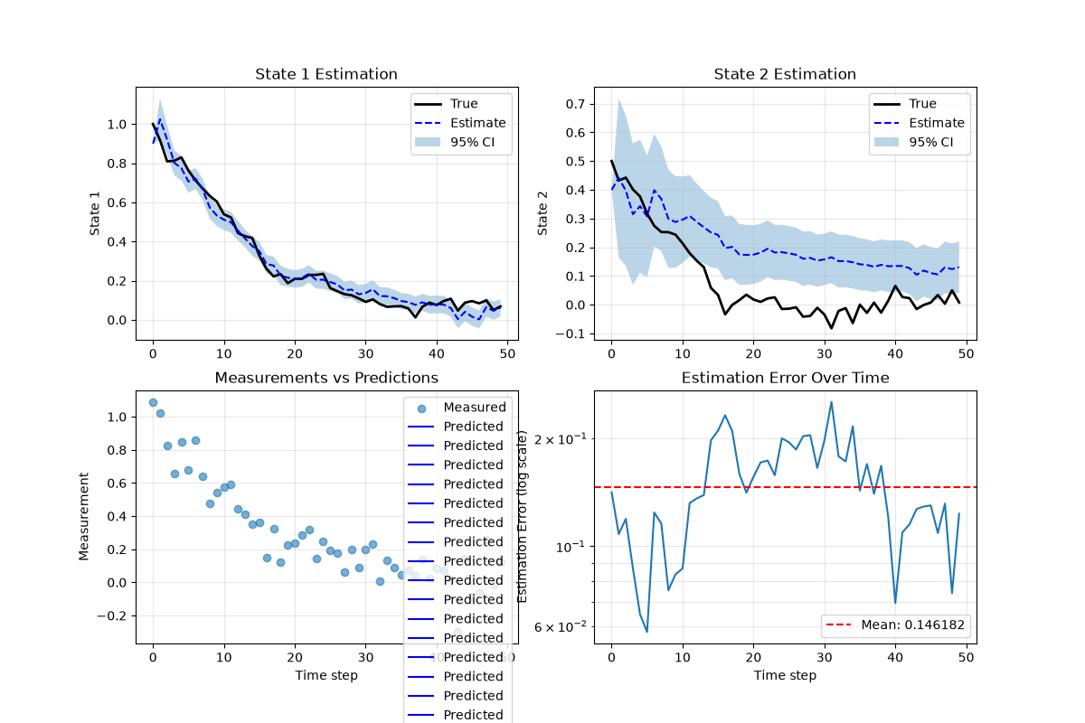
    fig, axes = plt.subplots(2, 2, figsize=(12, 8))

    # Plot 1: State estimates vs true state
    axes[0, 0].plot(x_true[:, 0], "k-", label="True", linewidth=2)
    axes[0, 0].plot(solution.x_plus[:, 0], "b--", label="Estimate", linewidth=1.5)
    axes[0, 0].fill_between(
        np.arange(n_timesteps),
        solution.x_plus[:, 0] - np.sqrt(np.diagonal(solution.Px_plus, axis1=1, axis2=2))[:, 0],
        solution.x_plus[:, 0] + np.sqrt(np.diagonal(solution.Px_plus, axis1=1, axis2=2))[:, 0],
        alpha=0.3,
        label="95% CI"
    )
    axes[0, 0].set_ylabel("State 1")
    axes[0, 0].legend()
    axes[0, 0].grid(True, alpha=0.3)
    axes[0, 0].set_title("State 1 Estimation")

    # Plot 2: Second state
    axes[0, 1].plot(x_true[:, 1], "k-", label="True", linewidth=2)
    axes[0, 1].plot(solution.x_plus[:, 1], "b--", label="Estimate", linewidth=1.5)
    axes[0, 1].fill_between(
        np.arange(n_timesteps),
        solution.x_plus[:, 1] - np.sqrt(np.diagonal(solution.Px_plus, axis1=1, axis2=2))[:, 1],
        solution.x_plus[:, 1] + np.sqrt(np.diagonal(solution.Px_plus, axis1=1, axis2=2))[:, 1],
        alpha=0.3,
        label="95% CI"
    )
    axes[0, 1].set_ylabel("State 2")
    axes[0, 1].legend()
    axes[0, 1].grid(True, alpha=0.3)
    axes[0, 1].set_title("State 2 Estimation")

    # Plot 3: Measurements
    axes[1, 0].scatter(np.arange(n_timesteps), y_meas[:, 0], alpha=0.6, label="Measured")
    axes[1, 0].plot(g(solution.x_plus.T), "b-", label="Predicted", linewidth=1.5)
    axes[1, 0].set_xlabel("Time step")
    axes[1, 0].set_ylabel("Measurement")
    axes[1, 0].legend()
    axes[1, 0].grid(True, alpha=0.3)
    axes[1, 0].set_title("Measurements vs Predictions")

    # Plot 4: Estimation error
    axes[1, 1].semilogy(state_error)
    axes[1, 1].axhline(y=mean_error, color="r", linestyle="--", label=f"Mean: {mean_error:.6f}")
    axes[1, 1].set_xlabel("Time step")
    axes[1, 1].set_ylabel("Estimation Error (log scale)")
    axes[1, 1].legend()
    axes[1, 1].grid(True, alpha=0.3, which="both")
    axes[1, 1].set_title("Estimation Error Over Time")

    plt.tight_layout()
    plt.savefig("kkf_basic_example.png", dpi=100, bbox_inches="tight")
    print("  Figure saved as 'kkf_basic_example.png'")

    plt.show()

    print("\n" + "=" * 70)
    print("Example completed successfully!")
    print("=" * 70)


if __name__ == "__main__":
    main()