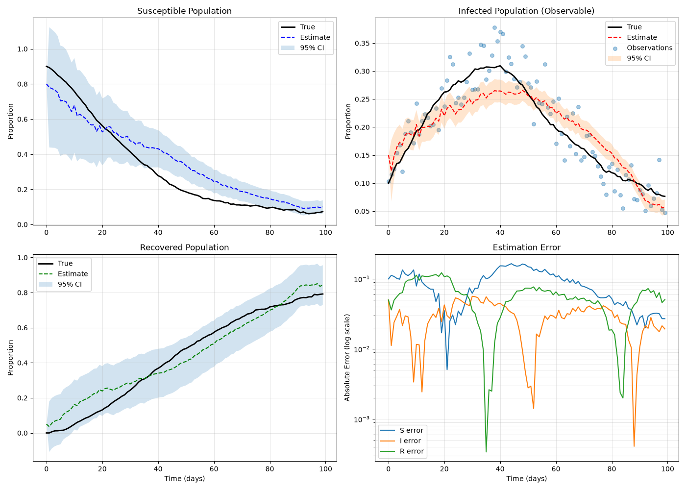
SIR Epidemic Model

This example demonstrates using KKF to estimate states in a Susceptible-Infected-Recovered (SIR) epidemiological model.

======================================================================
KKF Example: SIR Epidemiological Model
======================================================================

SIR Model Properties:
  Transmission rate (β): 0.12
  Recovery rate (γ): 0.04
  State dimension: 3 (S, I, R)
  Observable: Infected population

Generating synthetic epidemic data...
  Generated 100 timesteps
  Peak infected: 0.3095

Setting up Koopman Kalman Filter...
  Kernel: Matérn with length scale ~ 0.2714
  Number of features: 50
  Prior initial state: [0.8  0.15 0.05]

Applying Koopman Kalman Filter...
✓ Filter completed!

State Estimation Results:
  Initial S estimate: 0.8000 (true: 0.9000)
  Initial I estimate: 0.1500 (true: 0.1000)
  Initial R estimate: 0.0500 (true: 0.0000)

Generating plots...
  Figure saved as 'kkf_sir_example.png'

======================================================================
Example completed successfully!
======================================================================

import numpy as np
import matplotlib.pyplot as plt
from scipy import stats
from sklearn.gaussian_process.kernels import Matern

from kkf import DynamicalSystem, KoopmanOperator, apply_koopman_kalman_filter


def main():
    """Run SIR model KKF example."""
    print("=" * 70)
    print("KKF Example: SIR Epidemiological Model")
    print("=" * 70)

    # System parameters
    beta, gamma = 0.12, 0.04  # Transmission and recovery rates

    def f(x):
        """SIR dynamics."""
        return x + np.array([
            -beta * x[0] * x[1],
            beta * x[0] * x[1] - gamma * x[1],
            gamma * x[1]
        ])

    def g(x):
        """Observe infected population."""
        return np.array([x[1]])

    # System dimensions
    nx, ny = 3, 1
    n_features = 50

    # Noise distributions
    X_dist = stats.dirichlet(alpha=np.ones(nx))
    dyn_dist = stats.multivariate_normal(mean=np.zeros(nx), cov=1e-5 * np.eye(3))
    obs_dist = stats.multivariate_normal(mean=np.zeros(ny), cov=1e-3 * np.eye(1))

    # Create system
    system = DynamicalSystem(
        nx=nx,
        ny=ny,
        f=f,
        g=g,
        dist_X=X_dist,
        dist_dyn=dyn_dist,
        dist_obs=obs_dist,
        discrete_time=True,
    )

    print(f"\nSIR Model Properties:")
    print(f"  Transmission rate (β): {beta}")
    print(f"  Recovery rate (γ): {gamma}")
    print(f"  State dimension: {nx} (S, I, R)")
    print(f"  Observable: Infected population")

    # Generate synthetic data
    print(f"\nGenerating synthetic epidemic data...")
    n_timesteps = 100
    x_true = np.zeros((n_timesteps, nx))
    y_meas = np.zeros((n_timesteps, ny))

    # Initial condition: mostly susceptible, few infected
    x_true[0] = np.array([0.9, 0.1, 0.0])
    y_meas[0] = g(x_true[0]) + obs_dist.rvs()

    for t in range(1, n_timesteps):
        x_true[t] = f(x_true[t - 1]) + dyn_dist.rvs()
        # Ensure state remain in valid range [0, 1]
        x_true[t] = np.clip(x_true[t], 0, 1)
        y_meas[t] = g(x_true[t]) + obs_dist.rvs()

    print(f"  Generated {n_timesteps} timesteps")
    print(f"  Peak infected: {np.max(x_true[:, 1]):.4f}")

    # Setup Koopman operator
    print(f"\nSetting up Koopman Kalman Filter...")
    kernel = Matern(length_scale=n_features ** (-1 / nx), nu=0.5)
    koop = KoopmanOperator(kernel, system)

    # Prior distribution
    x0_prior = np.array([0.8, 0.15, 0.05])
    dist_prior = stats.multivariate_normal(mean=x0_prior, cov=0.1 * np.eye(3))

    print(f"  Kernel: Matérn with length scale ~ {kernel.length_scale:.4f}")
    print(f"  Number of features: {n_features}")
    print(f"  Prior initial state: {x0_prior}")

    # Apply filter
    print(f"\nApplying Koopman Kalman Filter...")
    solution = apply_koopman_kalman_filter(
        koopman_operator=koop,
        observations=y_meas,
        initial_distribution=dist_prior,
        n_features=n_features,
        optimize=False,
        noise_samples=100,
    )

    print(f"✓ Filter completed!")

    # Analysis
    print(f"\nState Estimation Results:")
    print(f"  Initial S estimate: {solution.x_plus[0, 0]:.4f} (true: {x_true[0, 0]:.4f})")
    print(f"  Initial I estimate: {solution.x_plus[0, 1]:.4f} (true: {x_true[0, 1]:.4f})")
    print(f"  Initial R estimate: {solution.x_plus[0, 2]:.4f} (true: {x_true[0, 2]:.4f})")

    # Visualization
    print(f"\nGenerating plots...")
    fig, axes = plt.subplots(2, 2, figsize=(14, 10))

    # Plot 1: Susceptible population
    time = np.arange(n_timesteps)
    axes[0, 0].plot(time, x_true[:, 0], "k-", label="True", linewidth=2)
    axes[0, 0].plot(time, solution.x_plus[:, 0], "b--", label="Estimate", linewidth=1.5)
    axes[0, 0].fill_between(
        time,
        solution.x_plus[:, 0] - 1.96 * np.sqrt(np.diagonal(solution.Px_plus, axis1=1, axis2=2))[:, 0],
        solution.x_plus[:, 0] + 1.96 * np.sqrt(np.diagonal(solution.Px_plus, axis1=1, axis2=2))[:, 0],
        alpha=0.2,
        label="95% CI"
    )
    axes[0, 0].set_ylabel("Proportion")
    axes[0, 0].set_title("Susceptible Population")
    axes[0, 0].legend()
    axes[0, 0].grid(True, alpha=0.3)

    # Plot 2: Infected population
    axes[0, 1].plot(time, x_true[:, 1], "k-", label="True", linewidth=2)
    axes[0, 1].plot(time, solution.x_plus[:, 1], "r--", label="Estimate", linewidth=1.5)
    axes[0, 1].scatter(time, y_meas[:, 0], alpha=0.4, s=30, label="Observations")
    axes[0, 1].fill_between(
        time,
        solution.x_plus[:, 1] - 1.96 * np.sqrt(np.diagonal(solution.Px_plus, axis1=1, axis2=2))[:, 1],
        solution.x_plus[:, 1] + 1.96 * np.sqrt(np.diagonal(solution.Px_plus, axis1=1, axis2=2))[:, 1],
        alpha=0.2,
        label="95% CI"
    )
    axes[0, 1].set_ylabel("Proportion")
    axes[0, 1].set_title("Infected Population (Observable)")
    axes[0, 1].legend()
    axes[0, 1].grid(True, alpha=0.3)

    # Plot 3: Recovered population
    axes[1, 0].plot(time, x_true[:, 2], "k-", label="True", linewidth=2)
    axes[1, 0].plot(time, solution.x_plus[:, 2], "g--", label="Estimate", linewidth=1.5)
    axes[1, 0].fill_between(
        time,
        solution.x_plus[:, 2] - 1.96 * np.sqrt(np.diagonal(solution.Px_plus, axis1=1, axis2=2))[:, 2],
        solution.x_plus[:, 2] + 1.96 * np.sqrt(np.diagonal(solution.Px_plus, axis1=1, axis2=2))[:, 2],
        alpha=0.2,
        label="95% CI"
    )
    axes[1, 0].set_ylabel("Proportion")
    axes[1, 0].set_xlabel("Time (days)")
    axes[1, 0].set_title("Recovered Population")
    axes[1, 0].legend()
    axes[1, 0].grid(True, alpha=0.3)

    # Plot 4: Phase portrait and error
    error_s = np.abs(solution.x_plus[:, 0] - x_true[:, 0])
    error_i = np.abs(solution.x_plus[:, 1] - x_true[:, 1])
    error_r = np.abs(solution.x_plus[:, 2] - x_true[:, 2])

    axes[1, 1].semilogy(time, error_s, label="S error", linewidth=1.5)
    axes[1, 1].semilogy(time, error_i, label="I error", linewidth=1.5)
    axes[1, 1].semilogy(time, error_r, label="R error", linewidth=1.5)
    axes[1, 1].set_xlabel("Time (days)")
    axes[1, 1].set_ylabel("Absolute Error (log scale)")
    axes[1, 1].set_title("Estimation Error")
    axes[1, 1].legend()
    axes[1, 1].grid(True, alpha=0.3, which="both")

    plt.tight_layout()
    plt.savefig("kkf_sir_example.png", dpi=100, bbox_inches="tight")
    print("  Figure saved as 'kkf_sir_example.png'")

    plt.show()

    print("\n" + "=" * 70)
    print("Example completed successfully!")
    print("=" * 70)


if __name__ == "__main__":
    main()